 Distribution Fitter: Introduction
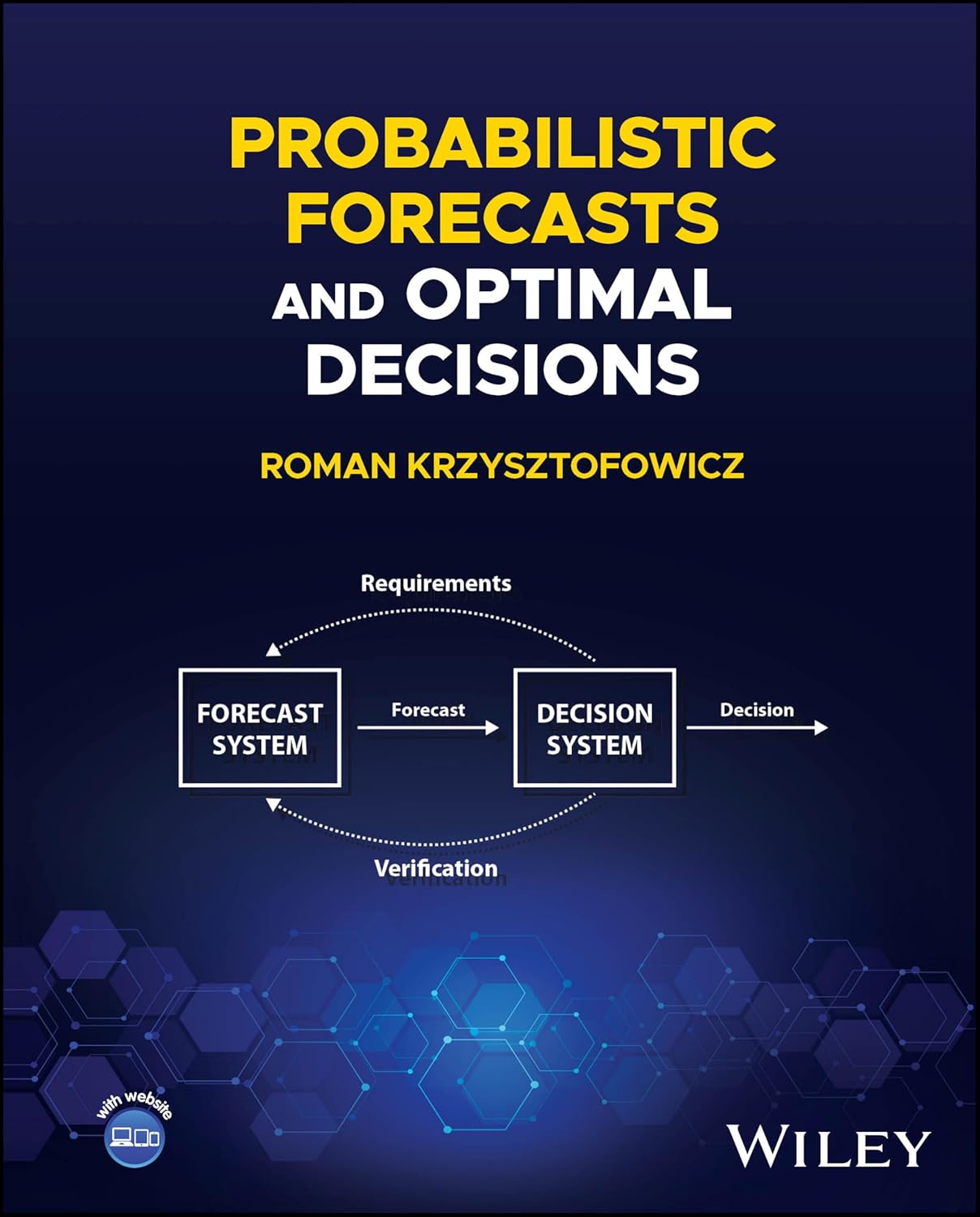
This web-based software accompanies the book Probabilistic Forecasts and Optimal Decisions authored by Roman Krzysztofowicz and published by Wiley in 2024.
Developed originally in 2003 as an aid to research, DFitTM implements a methodology for modeling probability distributions of continuous variates. It is a logical-statistical-numerical methodology that aids the user to hypothesize, estimate, evaluate, and choose a parametric distribution that best fits the data, which may come in either form:
- a random sample of realizations,
- a set of assessed quantiles.
This version of DFitTM offers 24 families of parametric distributions on 4 types of sample spaces. The allowable maximal (i) number of samples, (ii) sample size or number of quantiles, and (iii) number of fits depend on the license level (there are two).
The theory, procedures, and formulae (for the distribution functions, density functions, and quantile functions) are documented in the book, in:
Chapter 2. Basic Elements
Chapter 3. Distribution Modeling
Chapter 9. Judgmental Forecasting
Appendix B. Parameter Estimation Methods
Appendix C. Special Univariate Distributions
DFitTM is intended to be self-explanatory for a user who has the book and knows the above contents.
Notes on Numerical Procedures
1. Specifying the sample space.
When a bounded interval is specified, the initial bounds are displayed: eta L = smallest realization (or smallest quantile), eta U = largest realization (or largest quantile). These are merely aids to assessing the bounds via a logical analysis, as described in Section 3.3.2 of the book.
2. Pruning away identical realizations.
When there are 3 or more identical realizations (the ordinates) whose plotting positions (the abscissae) create a step in the empirical distribution function, only the middle abscissa (if their number is odd) or the two middle abscissae (if their number is even) are used in the estimation of parameters.
3. Calculating maximum absolute difference,
MAD.
This is done using the pruned empirical distribution function. Thus, the
MAD measures the goodness of fit of a given parametric distribution function relative to the best feasible fit (MAD=0), which a continuous strictly increasing function passing through the midpoints of abscissae would offer. Consequently, when the steps created by abscissae of identical realizations are high, the MAD may be significantly smaller than the K-S statistic D, which is calculated using the entire empirical distribution function.
4. Calculating critical value C for the K-S test.
This C is taken from Table 3.2 in the book for sample sizes N = 2, 3, 4, 5, and is calculated via a custom algorithm for any N > 5. The calculated and the tabulated C may differ slightly. The reported significance level 0.00 means that the model is rejected at the significance level 0.01.
User Instructions
Creating an Account and Subscribing
Create an Account
First time user: choose the "sign up" option on the login page to register an account with F-D Systems. Instructor or Student: use your school email address. A strong password is recommended.
Choose a Subscription
The first time you login, before you can use DFitTM, you will be prompted to select a subscription license. There are two levels:
| Academic License | Professional License | |
|---|---|---|
| Description | Instructor or Student | Researcher or Analyst |
| Fee | $5 / 6 months | $19 / 6 months |
| Max Number of Samples | 30 | 100 |
| Max Sample Size | 150 | 5,000 |
| Max Number of Fits | 900 | 3,000 |
| Renewals | Instructor: unlimited Student: one-time | unlimited |
Limit of Liability / Disclaimer of Warranty
The author of the book and the developers of the DFitTM software have made reasonable efforts to ensure the quality and reliability of the information and tools provided. However, DFitTM is provided “as is” and “as available” without warranties of any kind, express or implied, including but not limited to warranties of merchantability, fitness for a particular purpose, non-infringement, accuracy, completeness, or reliability of outputs or results.
No oral or written information, promotional material, review, or commentary shall create any warranty or representation unless expressly stated in writing by an authorized representative.
You are solely responsible for how you use the software and any decisions or actions you take based upon its outputs. The software may not be suitable for your particular needs or situation.
To the maximum extent permitted by law, the author and the developers shall not be liable for any direct, indirect, incidental, special, consequential, or exemplary damages, including but not limited to loss of profits, loss of data, or business interruption, arising from or relating to the use of or inability to use DFitTM, even if advised of the possibility of such damages.
Using DFitTM
Go to "My Samples" and "Create New Sample and Specs"
In the box "Create Sample and Specs":
| Sample data file | Upload the file containing your data: "CSV" file, without header, with one or two columns (see Data type) | ||||
| Name | Name your file | ||||
| Data type | Select type that is compatible with the data file:
|
||||
| Plotting positions | Select formula (only when "Random Sample"): "Meta-Gaussian" should be used for exercises and mini-projects |
||||
| Bounds on sample space | Specify the type of sample space Assess the bounds |
||||
| Hypothesized distributions | Select the distribution families (only those catalogued in Appendix C, or Gaussian from Chapter 2) |
Go to "Create"
Request "Statistics and Fit", or "Duplicate" the sample, or "Edit" the specs, or "Delete" the sample
| "Perform Fit" | Estimates parameters and calculates MAD |
| "View Fits" | Displays a table with parameter estimates and MAD values The distributions can be ordered according to a column values |
| "Download Fits" | Downloads parameter estimates and MAD values |
Limitation
One set of specs per sample. Thus, if after the fit you want to modify the specs and redo the fit,
then you need to "Duplicate" the sample, "Edit" the specs, and select anew the hypothesized
distribution families.
Probabilistic Forecasts and Optimal Decisions
By Roman Krzysztofowicz, Wiley 2024
Chapter Headings
1. FORECAST—DECISION THEORY
Part one: Elements of Probability
2. BASIC ELEMENTS
3. DISTRIBUTION MODELING
Part two: Discrete Models
4. JUDGMENTAL FORECASTING
5. STATISTICAL FORECASTING
6. VERIFICATION OF FORECASTS
7. DETECTION-DECISION THEORY
8. VARIOUS DISCRETE MODELS
Part three: Continuous Models
9. JUDGMENTAL FORECASTING
10. STATISTICAL FORECASTING
11. VERIFICATION OF FORECASTS
12. TARGET-DECISION THEORY
13. INVENTORY AND CAPACITY MODELS
14. INVESTMENT MODELS
15. VARIOUS CONTINUOUS MODELS
Appendices
A. RATIONALITY POSTULATES
B. PARAMETER ESTIMATION METHODS
C. SPECIAL UNIVARIATE DISTRIBUTIONS
From Wiley Editor
Account for uncertainties and optimize decision-making with this thorough exposition
Decision theory is a body of thought and research seeking to apply a mathematical-logical framework to assessing probability and optimizing decision-making. It has developed robust tools for addressing all major challenges to decision making. Yet the number of variables and uncertainties affecting each decision outcome, many of them beyond the decider's control, mean that decision-making is far from a 'solved problem'. The tools created by decision theory remain to be refined and applied to decisions in which uncertainties are prominent.
Probabilistic Forecasts and Optimal Decisions introduces a theoretically-grounded methodology for optimizing decision-making under conditions of uncertainty. Beginning with an overview of the basic elements of probability theory and methods for modeling continuous variates, it proceeds to survey the mathematics of both continuous and discrete models, supporting each with key examples. The result is a crucial window into the complex but enormously rewarding world of decision theory.
Probabilistic Forecasts and Optimal Decisions readers will also find:
- Extended case studies supported with real-world data
- Mini-projects running through multiple chapters to illustrate different stages of the decision-making process
- End of chapter exercises designed to facilitate student learning
Probabilistic Forecasts and Optimal Decisions is ideal for advanced undergraduate and graduate students in the sciences and engineering, as well as predictive analytics and decision analytics professionals.